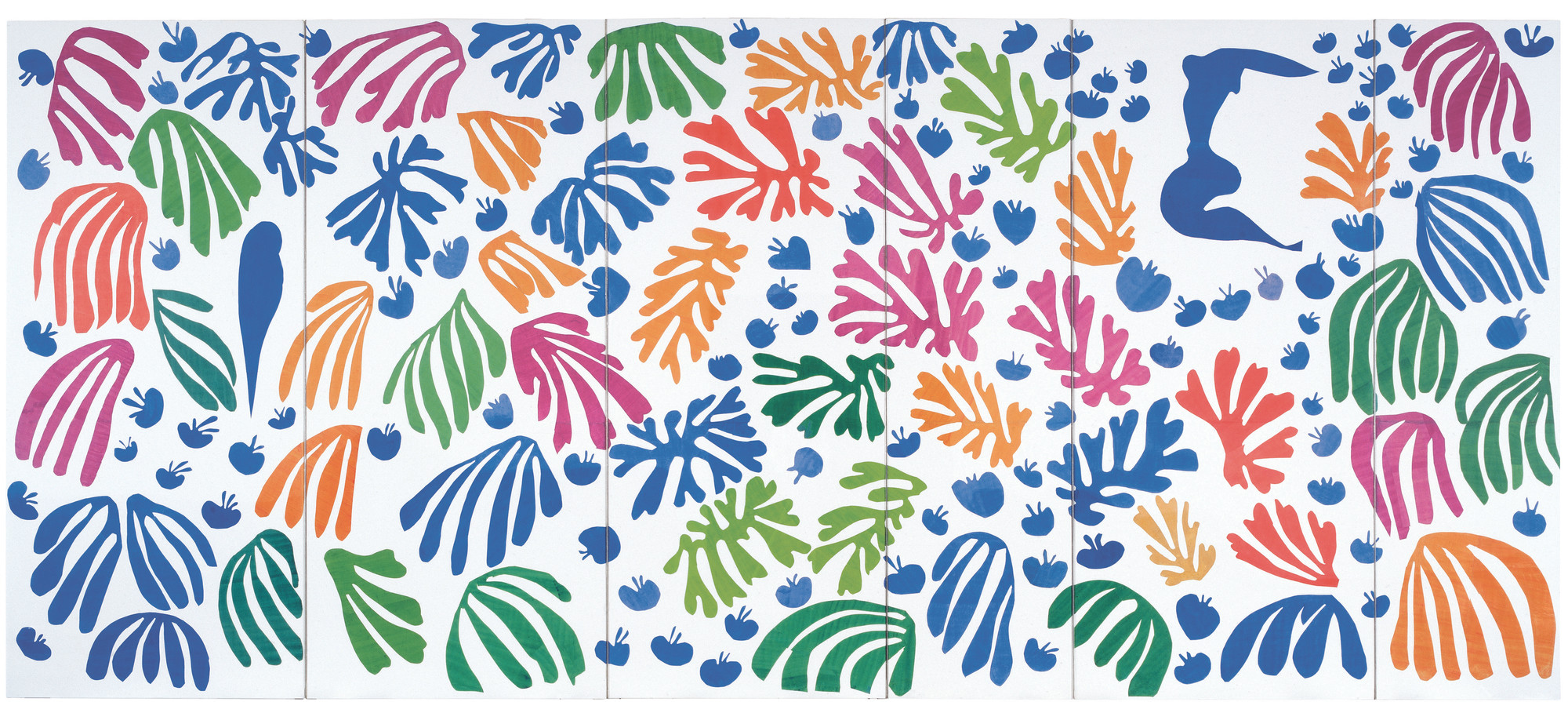
3.3. ECT on Matisse’s “The Parakeet and the Mermaid”

Here, we are going to give an example of using the ECT to classify the cutout shapes from Henri Matisse’s 1952 “The Parakeet and the Mermaid”.

# -----------------
# Standard imports
# -----------------
import numpy as np  # for arrays
import matplotlib.pyplot as plt  # for plotting
from sklearn.decomposition import PCA  # for PCA for normalization
from scipy.spatial import distance_matrix

from os import listdir  # for retrieving files from directory
from os.path import isfile, join  # for retrieving files from directory
from sklearn.manifold import MDS  # for MDS
import pandas as pd  # for loading in colors csv
import os
import zipfile

import warnings
warnings.filterwarnings('ignore')

# ---------------------------
# The ECT packages we'll use
# ---------------------------
from ect import ECT, EmbeddedGraph  # for calculating ECTs

# Simple data paths
data_dir = "outlines/"
colors_path = "colors.csv"

file_names = [
    f for f in listdir(data_dir) if isfile(join(data_dir, f)) and f[-4:] == ".txt"
]
file_names.sort()
print(f"There are {len(file_names)} files in the directory")

There are 150 files in the directory

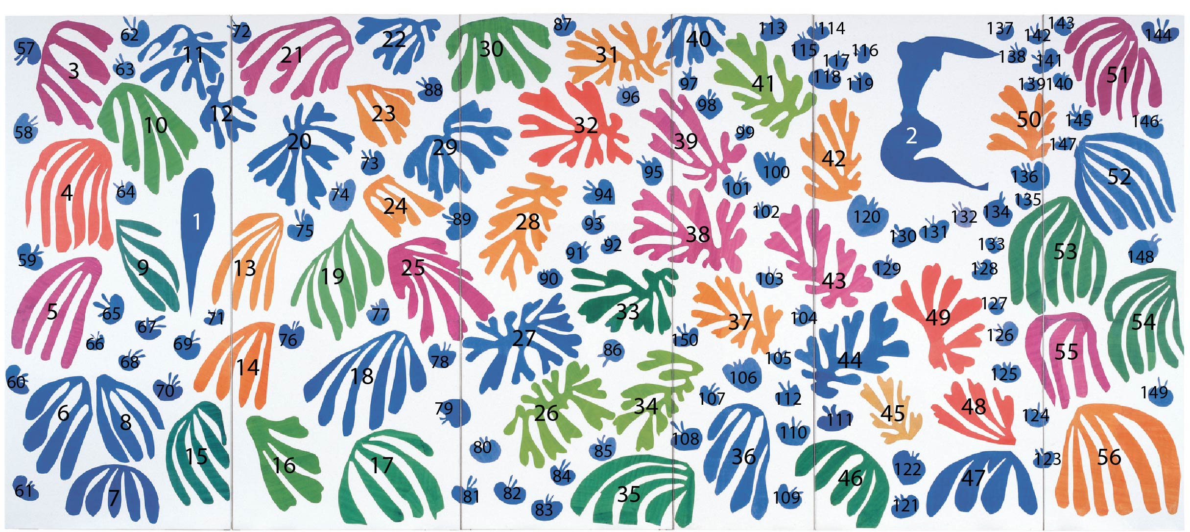
We’ve taken care of the preprocessing in advance by extracting out the shapes from the image. You can download these outlines here: outlines.zip.

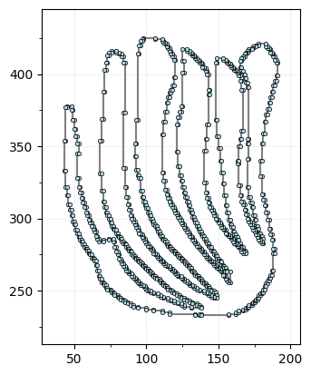
i = 3
shape = np.loadtxt(data_dir + file_names[i])
# shape = normalize(shape)
G = EmbeddedGraph()
G.add_cycle(shape)
G.plot(with_labels=False, node_size=10)

<Axes: >

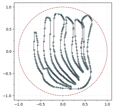
We’re going to align the leaf using the PCA coordinates, min-max center, and scale it to fit in a ball of radius 1 for ease of comparisons.

G.transform_coordinates(projection_type="pca")  # project with PCA
G.scale_coordinates(1)  # scale to radius 1
G.plot(with_labels=False, node_size=10, bounding_circle=True)

<Axes: >

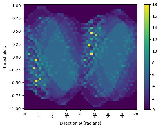
And then we can compute the ECT of this leaf.

num_dirs = 50  # set number of directional axes
num_thresh = 50  # set number of thresholds each axis

myect = ECT(num_dirs=num_dirs, num_thresh=num_thresh);  # intiate ECT
result = myect.calculate(G);  # calculate ECT on embedded graph

result.plot();  # plot ECT

OMP: Info #276: omp_set_nested routine deprecated, please use omp_set_max_active_levels instead.

Let’s just make a data loader with all of this for ease in a bit.

def matisse_ect(filename, ect):
    shape = np.loadtxt(data_dir + filename)
    G = EmbeddedGraph()
    G.add_cycle(shape)
    G.transform_coordinates(projection_type="pca")
    G.scale_coordinates(1)
    result = ect.calculate(G)
    return result

And now we can load in all the outlines, compute their ECT and store it in a 3D array.

num_dirs = 50  # set number of directional axes
num_thresh = 50  # set number of thresholds each axis

ect_arr = np.zeros((len(file_names), num_dirs, num_thresh))
myect = ECT(num_dirs=num_dirs, num_thresh=num_thresh, bound_radius=1)

for i in range(len(file_names)):  # for each leaf
    ect_arr[i, :, :] = matisse_ect(file_names[i], myect)

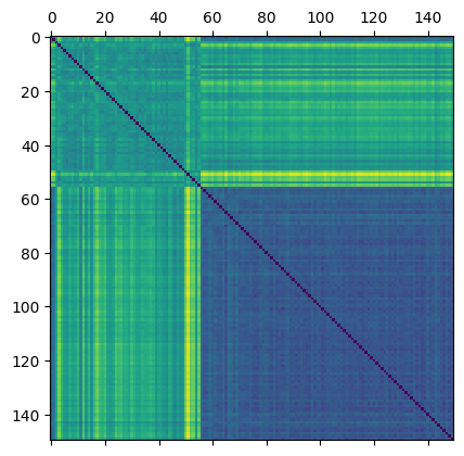
Here, we are just going to compute the distance between two ECTs using \(L_2\) distance.

flattened_ect = ect_arr.reshape(len(file_names), num_dirs * num_thresh)
D = distance_matrix(flattened_ect, flattened_ect)
plt.matshow(D)

<matplotlib.image.AxesImage at 0x32185cbd0>

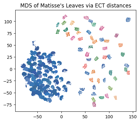
For visualization purposes, we can project this data into 2D using Multi Dimensional Scaling (MDS). Here we plot each figure at the MDS coordinates.

n_components = 2  # select number of components
mds = MDS(
    n_components=n_components,  # initialize MDS
    dissimilarity="precomputed",  # we have precomputed the distance matrix
    normalized_stress="auto",
    random_state=5,  # select random state for reproducibility
)
MDS_scores = mds.fit_transform(D)  # get MDS scores

# read in color hexcodes
col_df = pd.read_csv(colors_path, header=None)

scale_val = 6  # set scale value
plt.figure(figsize=(5, 5))  # set figure dimensions

for i in range(len(file_names)):  # for each leaf
    shape = np.loadtxt(data_dir + file_names[i])  # get the current shape
    shape = shape - np.mean(shape, axis=0)  # zero center shape
    shape = (
        scale_val * shape / max(np.linalg.norm(shape, axis=1))
    )  # scale to radius 1 then mult by scale_val

    trans_sh = shape + MDS_scores[i]  # translate shape to MDS position

    plt.fill(trans_sh[:, 0], trans_sh[:, 1], c=col_df[0][i], lw=0)  # plot shape
    plt.gca().set_aspect("equal")

plt.title("MDS of Matisse's Leaves via ECT distances")
# plt.savefig("Matisse_MDS.png", bbox_inches = 'tight', dpi=300)

Text(0.5, 1.0, "MDS of Matisse's Leaves via ECT distances")

3.3.1. Acknowledgements

This notebook was written by Liz Munch based on original code from Dan Chitwood.