7. Computing the Reeb graph of a filtered simplicial complex

This notebook gives a tutorial to computing the Reeb graph from a filtered simplicial complex. We assume that this complex is given as the LowerStar class (see LowerStar documentation for details).

from cereeberus import LowerStar, ReebGraph, computeReeb

7.1. Simple example

Consider the following simplicial complex with height function.

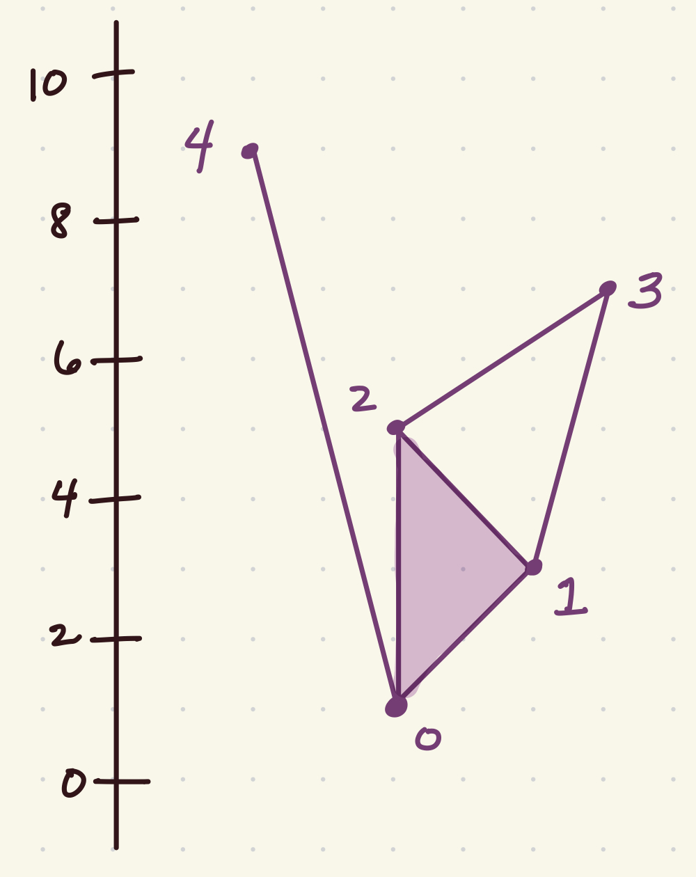
First, we construct this simplicial complex with a lower star filtration, were we need only specify the top dimensional simplices. Note that the LowerStar class is built on gudhi’s SimplexTree, so it retains all of that class’ functionality.

K = LowerStar()
K.insert([0, 1, 2])
K.insert([1, 3])
K.insert([2,3])
K.insert([0,4])
K.assign_filtration([0], 0.0)
K.assign_filtration([1], 3.0)
K.assign_filtration([2], 5.0)
K.assign_filtration([3], 7)
K.assign_filtration([4], 9.0)

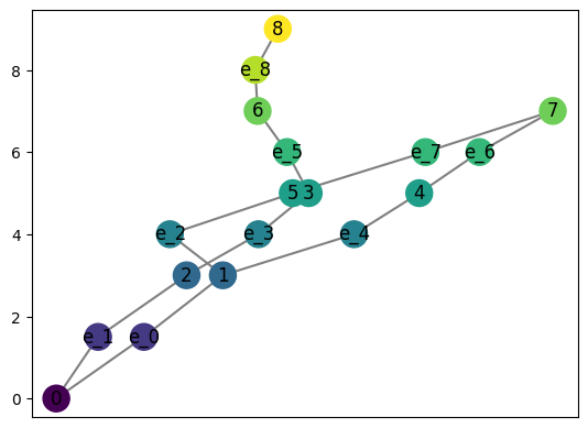
Then computing the Reeb graph of this complex is as easy as the following. By default, the Reeb graph only has nodes where the topology of the level sets changes: minima, maxima, and the points where components merge or split. Here the minimum at height 0 has two edges going up: one to the maximum at height 9 (vertex 4), and one to a split at height 3. The two edges from the split meet again at height 7, forming a loop. (cpx controls how far apart parallel edges are drawn.)

R = computeReeb(K)
R.draw(cpx=1)

7.1.1. Keeping the regular nodes

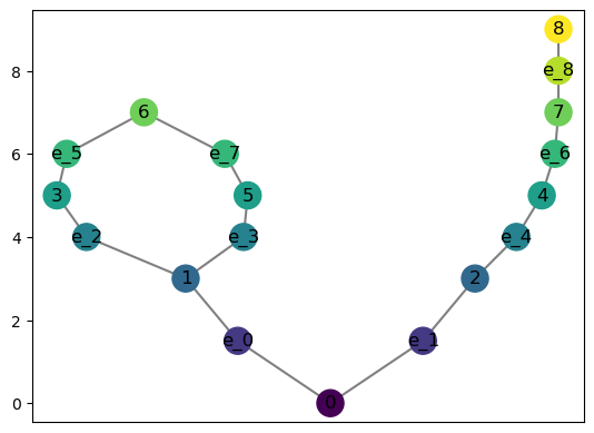
Nodes with exactly one edge coming in from below and one going out above are regular: the level set does not change there, so they are not needed to describe the Reeb graph. They are left out by default. To keep a node for every level-set component at every vertex height, with a midpoint node (named e_0, e_1, …) on each edge in between, pass keep_regular_nodes=True. This is the output format of cereeberus 0.1.20 and earlier.

Both graphs describe the same Reeb graph; the second one just subdivides its edges.

R_full = computeReeb(K, keep_regular_nodes=True)
print('default:', R.number_of_nodes(), 'nodes,', R.number_of_edges(), 'edges')
print('keep_regular_nodes:', R_full.number_of_nodes(), 'nodes,', R_full.number_of_edges(), 'edges')
R_full.draw()

default: 4 nodes, 4 edges
keep_regular_nodes: 18 nodes, 18 edges

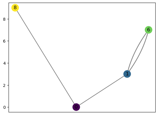
Going the other way, remove_all_regular_vertices removes the regular nodes from a graph that has them, which recovers the default output.

R_full.remove_all_regular_vertices()
R_full.draw()

7.2. Torus example

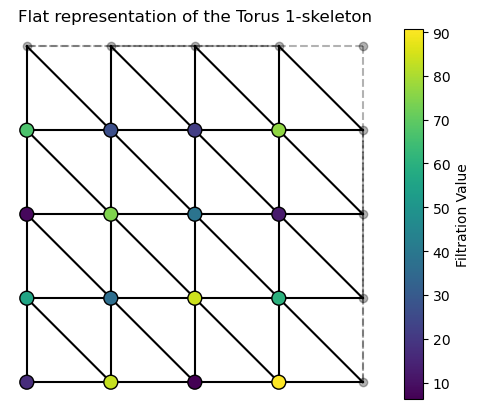
For a slightly more complex example, we have the following Torus example generator.

from cereeberus.data import Torus

T = Torus()
T.generate_grid(grid_size = 4)
T.assign_random_values(0,100, seed=1986)
T.draw()

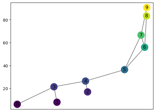
R = computeReeb(T)

R.draw(cpx = 2)

7.3. Degenerate (horizontal) edges

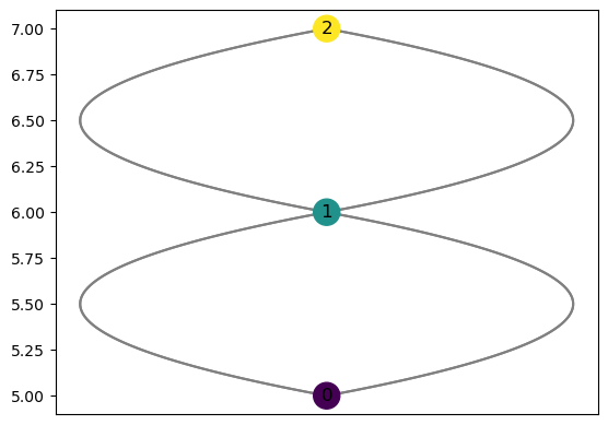
Here we check an example where there might be a horizontal edge in the input filtered simplicial complex which should end up being collapsed in the resulting Reeb graph.

K = LowerStar()
K.insert([0,1])
K.insert([0,2])
K.insert([1,2])
K.insert([1,3])
K.insert([2,3])
K.assign_filtration([0], 5.0)
K.assign_filtration([1], 6.0)
K.assign_filtration([2], 6.0)
K.assign_filtration([3], 7)

R = computeReeb(K)
R.draw()

7.4. Higher-dimensional complexes

computeReeb works for complexes of any dimension. As an example, a solid tetrahedron with a height function has a Reeb graph that is a single edge, because every level set is connected.

K = LowerStar()
K.insert([0, 1, 2, 3])
for v, height in enumerate([0.0, 1.0, 2.0, 3.0]):
    K.assign_filtration([v], height)

R = computeReeb(K)
R.draw()

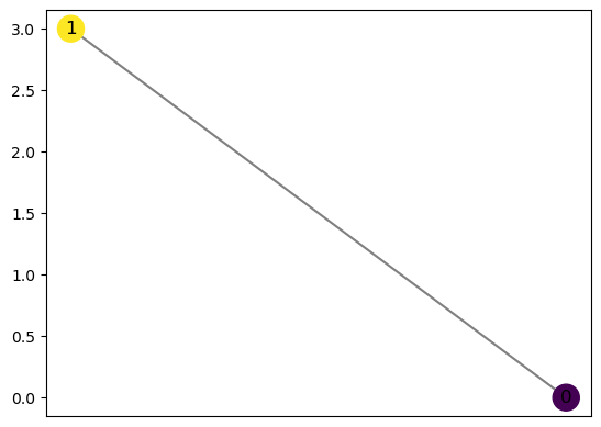
Only the vertices, edges and triangles are needed to compute a Reeb graph, so the higher-dimensional simplices do not slow down the computation.

7.5. Large complexes

For large complexes, such as surface meshes with many thousands of vertices, a few options can help:

• set_pos=False skips computing a drawing layout. Call R.set_pos_from_f() later if you want to draw the graph.

• validate=False skips checking that the filtration of every simplex is the maximum of its vertex values. LowerStar maintains this automatically, so the check can be skipped for complexes built with assign_filtration.

• verbose=True prints progress as the computation sweeps through the vertex heights.

R = computeReeb(K, set_pos=False, validate=False, verbose=True)