3.4. Tutorial for exact ECT computation

Warning: This is a work in progress. Proceed at your own risk.

The goal of this section is so show available tools for exact computation of the ECT.

from ect import ECT, EmbeddedGraph, EmbeddedCW,create_example_graph

import matplotlib.pyplot as plt
from matplotlib.patches import Circle
import numpy as np
import networkx as nx

We can use the EmbeddedGraph class to find the angle normal to any pair of vertices in the graph, whether or not there is a connecting edge. Setting angle_labels_circle=True in the plotting command will try to draw these on the circle. Note that this doesn’t tend to do well for large inputs, but can be helpful for small examples.

# Super simple graph
G = EmbeddedGraph()
G.add_node('A', 0,0)
G.add_node('B', 1,0)
G.add_node('C', 2,1)
G.add_node('D', 1,2)
G.add_edge('A', 'B')
G.add_edge('B', 'D')
G.add_edge('D', 'C')

fig, ax = plt.subplots()
G.plot(ax = ax)
G.plot_angle_circle(ax = ax)

G = create_example_graph(centered=True)
G.rescale_to_unit_disk()


fig, ax = plt.subplots()
G.plot(ax = ax)
G.plot_angle_circle(ax = ax)

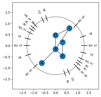
We can extract the information directly for use in computation.

# If return type is `matrix`, the function returns the matrix of angles and the labels of the angles in the order of the rows/columns in the matrix
M,Labels = G.get_all_normals_matrix()
print(M)

plt.matshow(M)
plt.xticks(range(len(Labels)), Labels)
plt.yticks(range(len(Labels)), Labels)
plt.colorbar()

[[       nan 5.49778714 5.60844436 5.8195377  5.03413953 5.49778714]
 [2.35619449        nan 5.6951827  0.         3.92699082 5.49778714]
 [2.46685171 2.55359005        nan 2.03444394 2.89661399 2.67794504]
 [2.67794504 3.14159265 5.17603659        nan 3.46334321 3.92699082]
 [1.89254688 0.78539816 6.03820664 0.32175055        nan 0.        ]
 [2.35619449 2.35619449 5.8195377  0.78539816 3.14159265        nan]]

<matplotlib.colorbar.Colorbar at 0x16b198290>

This can also be returned as a dictionary, with keys given by angles (note the negative angle is not repeated), and value a list of the pairs of vertices associated. Note that in the case of more than one pair of vertices having the same normal angle, it is given as a list of all pairs.

angles_dict = G.get_normals_dict()
angles_dict

{5.497787143782138: [('A', 'B'), ('A', 'F'), ('B', 'F')],
 5.608444364956034: [('A', 'C')],
 5.81953769817878: [('A', 'D'), ('F', 'C')],
 5.034139534781332: [('A', 'E')],
 5.695182703632018: [('B', 'C')],
 0.0: [('B', 'D'), ('E', 'F')],
 3.9269908169872414: [('B', 'E'), ('D', 'F')],
 2.0344439357957027: [('C', 'D')],
 2.896613990462929: [('C', 'E')],
 3.4633432079864352: [('D', 'E')]}

We can also get it to return the dictionary with rounded values, as well as to have it include all the opposite angles.

G.get_normals_dict(opposites = True,
                   num_rounding_digits=2)

{5.5: [('A', 'B'), ('A', 'F'), ('B', 'F')],
 5.61: [('A', 'C')],
 5.82: [('A', 'D'), ('F', 'C')],
 5.03: [('A', 'E')],
 5.7: [('B', 'C')],
 0.0: [('B', 'D'), ('E', 'F')],
 3.93: [('B', 'E'), ('D', 'F')],
 2.03: [('C', 'D')],
 2.9: [('C', 'E')],
 3.46: [('D', 'E')],
 2.36: [('A', 'B'), ('A', 'F'), ('B', 'F')],
 2.47: [('A', 'C')],
 2.68: [('A', 'D'), ('F', 'C')],
 1.89: [('A', 'E')],
 2.56: [('B', 'C')],
 3.14: [('B', 'D'), ('E', 'F')],
 0.79: [('B', 'E'), ('D', 'F')],
 5.17: [('C', 'D')],
 6.04: [('C', 'E')],
 0.32: [('D', 'E')]}