9. Tutorial: Branch Decomposition of a Reeb Graph

A branch decomposition breaks a Reeb graph into a collection of non-overlapping upward paths called branches. Each branch travels strictly upward in function value, starting at either a local minimum or a saddle point and ending at either a local maximum or another saddle point.

Each branch stores:

• The function values at its two endpoints (f_low, f_high)

• Attachment information: which earlier branch each endpoint belongs to (pointing to itself if it is a local min/max)

This tutorial follows the branch decomposition definition from Samira Jabry’s thesis, Unsmoothing of Reeb Graphs, Saint Louis University, 2025. Further developments will be presented in forthcoming work.

For the API and class reference, see the branch decomposition documentation page.

import matplotlib.pyplot as plt

from cereeberus import ReebGraph
import cereeberus.data.ex_reebgraphs as ex_rg
from cereeberus.reeb.branchdecomp import BranchDecomp

9.1. A simple example: the dancing man

We’ll start with the dancing_man example graph, which is a connected Reeb graph with several saddle points.

R = ex_rg.dancing_man()

fig, axes = plt.subplots(1, 2, figsize=(14, 6))
R.draw(ax=axes[0])
axes[0].set_title('Reeb Graph', fontsize=14, fontweight='bold')

bd = R.branch_decomp()
bd.draw(ax=axes[1])

plt.tight_layout()
plt.show()

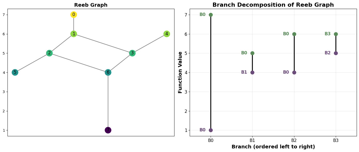
The branch decomposition diagram shows each branch as a vertical line positioned at its function values. Labels next to each endpoint indicate which branch that endpoint is attached to:

• Purple (lower endpoint): the branch ID whose path contains this vertex

• Green (upper endpoint): the branch ID whose path contains this vertex

When a label matches the branch’s own ID, that endpoint is a local min or max (no other branch claims it).

9.2. Inspecting the branches

The branches are stored as an \(n \times 4\) numpy array. Each row is one branch:

Column	Meaning
0	f_low — function value of the lower endpoint
1	f_high — function value of the upper endpoint
2	low_attach — branch ID owning the lower endpoint
3	high_attach — branch ID owning the upper endpoint

print("Branches (f_low, f_high, low_attach, high_attach):")
print(bd.branches)

Branches (f_low, f_high, low_attach, high_attach):
[[1. 7. 0. 0.]
 [4. 5. 1. 0.]
 [4. 6. 0. 0.]
 [5. 6. 2. 3.]]

# You can also inspect individual branches and their vertex paths
for i in range(len(bd.branches)):
    print(f"Branch {i}: f=[{bd.branches[i,0]}, {bd.branches[i,1]}]  "
          f"attaches=({int(bd.branches[i,2])}, {int(bd.branches[i,3])})  "
          f"path={bd.get_branch_path(i)}")

Branch 0: f=[1.0, 7.0]  attaches=(0, 0)  path=[7, 6, 2, 1, 0]
Branch 1: f=[4.0, 5.0]  attaches=(1, 0)  path=[5, 2]
Branch 2: f=[4.0, 6.0]  attaches=(0, 0)  path=[6, 3, 1]
Branch 3: f=[5.0, 6.0]  attaches=(2, 3)  path=[3, 4]

9.3. Reconstructing the Reeb graph

Once you have a branch decomposition, you can reconstruct the original Reeb graph exactly from it using reconstruct().

R2 = bd.reconstruct()

fig, axes = plt.subplots(1, 2, figsize=(12, 5))
R.draw(ax=axes[0])
axes[0].set_title('Original', fontsize=13, fontweight='bold')
R2.draw(ax=axes[1])
axes[1].set_title('Reconstructed', fontsize=13, fontweight='bold')
plt.tight_layout()
plt.show()

print(f"Original:      {R}")
print(f"Reconstructed: {R2}")

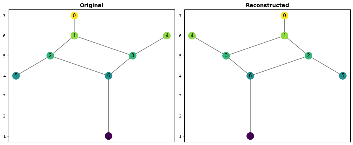
Original:      ReebGraph with 8 nodes and 8 edges.
Reconstructed: ReebGraph with 8 nodes and 8 edges.

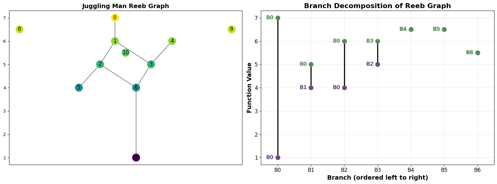
9.4. Handling isolated vertices: the juggling man

The juggling_man graph has isolated vertices (vertices with no edges), representing disconnected components. These are handled as degenerate branches where f_low == f_high and both attachment IDs point to the branch itself.

J = ex_rg.juggling_man()

fig, axes = plt.subplots(1, 2, figsize=(16, 6))
J.draw(ax=axes[0])
axes[0].set_title('Juggling Man Reeb Graph', fontsize=14, fontweight='bold')

bd_j = J.branch_decomp()
bd_j.draw(ax=axes[1])

plt.tight_layout()
plt.show()

# Identify the degenerate branches (isolated vertices)
print("Degenerate branches (isolated vertices):")
for i, (f_low, f_high, low_a, high_a) in enumerate(bd_j.branches):
    if f_low == f_high:
        print(f"  Branch {i}: vertex={bd_j.get_branch_path(i)}, f={f_low}, "
              f"attaches=({int(low_a)}, {int(high_a)})")

Degenerate branches (isolated vertices):
  Branch 4: vertex=[8], f=6.5, attaches=(4, 4)
  Branch 5: vertex=[9], f=6.5, attaches=(5, 5)
  Branch 6: vertex=[10], f=5.5, attaches=(6, 6)

9.5. Summary

The BranchDecomp class provides:

• decompose(R) — compute the decomposition from a ReebGraph

• branches — the \(n \times 4\) array of branch data

• get_branch(i) — return row \(i\) of the branches array

• get_branch_path(i) — return the list of vertices in branch \(i\)

• reconstruct() — rebuild the original ReebGraph from the stored paths

• draw() — visualise the decomposition

You can also call R.branch_decomp() directly on any ReebGraph or MapperGraph as a shortcut.