3.1. Tutorial: ECT for Embedded Cell Complexes

This tutorial will walk you through using the ECT package. Particularly we will show the features of EmbeddedComplex class for computing the Euler Characteristic Transform on complexes with arbitrary dimensional cells.

The EmbeddedComplex class combines and extends the functionality of the previous EmbeddedGraph and EmbeddedCW classes, supporting k-cells for k ≥ 2.

import numpy as np
import matplotlib.pyplot as plt
from ect import EmbeddedComplex, ECT, Directions
from ect.utils.examples import create_example_graph, create_example_cw, create_example_3d_complex

3.1.1. Basic Usage: Creating Simple Complexes

3.1.1.1. Example 1: Graph (1-skeleton)

Let’s start with a simple triangle graph (for legacy users this can be equivalently done using EmbeddedGraph).

K = EmbeddedComplex()

K.add_node('A', [0, 0])
K.add_node('B', [1, 0])
K.add_node('C', [0.5, 0.866])

K.add_edge('A', 'B')
K.add_edge('B', 'C')
K.add_edge('C', 'A')

#using built-in plotting function along with matplotlib
fig, ax = plt.subplots(figsize=(6, 6))
K.plot(ax=ax, with_labels=True, node_size=400)
ax.set_title('Simple Triangle Graph\n(0-cells: vertices, 1-cells: edges)')
plt.show()

#print some information about the complex
print(f"Number of nodes: {len(K.nodes())}")
print(f"Number of edges: {len(K.edges())}")
print(f"Embedding dimension: {K.dim}")

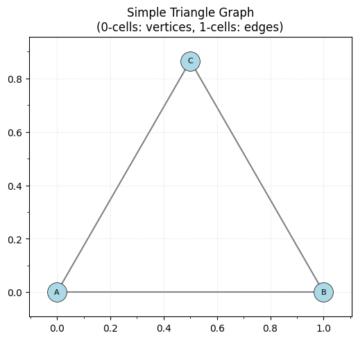
Number of nodes: 3
Number of edges: 3
Embedding dimension: 2

Now let’s add a 2-cell (face) to fill in the triangle:

K.add_face(['A', 'B', 'C'])

fig, ax = plt.subplots(figsize=(6, 6))
K.plot(ax=ax, with_labels=True, node_size=400, face_alpha=0.3, face_color='lightblue')
ax.set_title('Triangle with Face\n(0-cells: vertices, 1-cells: edges, 2-cells: faces)')
plt.show()

print(f"Number of 2-cells (faces): {len(K.faces)}")
print(f"Faces: {K.faces}")
print(f"Internal cells dictionary: {dict(K.cells)}")

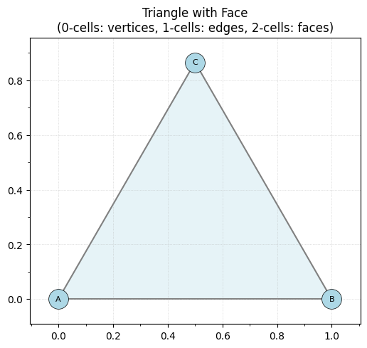
Number of 2-cells (faces): 1
Faces: [('A', 'B', 'C')]
Internal cells dictionary: {2: [(0, 1, 2)]}

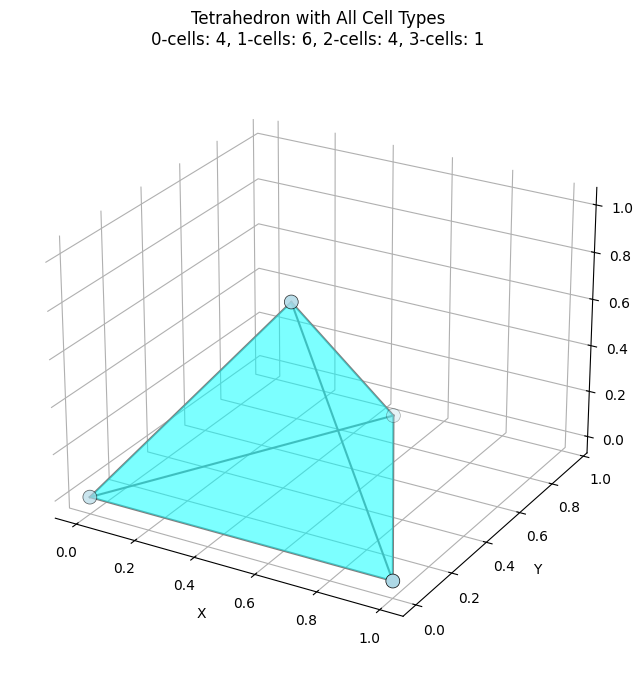
3.1.2. Adding Cells of Arbitrary Dimension

The key new feature is the ability to add cells of any dimension:

# Create a 3D tetrahedron with 0, 1, 2, and 3-cells
K_tetra = EmbeddedComplex()

# Add vertices (0-cells)
vertices = {
    'A': [0, 0, 0],
    'B': [1, 0, 0],
    'C': [0.5, 0.866, 0],
    'D': [0.5, 0.289, 0.816]
}

for name, coord in vertices.items():
    K_tetra.add_node(name, coord)

# Add edges (1-cells) - all pairs
edges = [('A', 'B'), ('A', 'C'), ('A', 'D'), ('B', 'C'), ('B', 'D'), ('C', 'D')]
K_tetra.add_edges_from(edges)

# Add faces (2-cells) - all triangular faces
faces = [['A', 'B', 'C'], ['A', 'B', 'D'], ['A', 'C', 'D'], ['B', 'C', 'D']]
for face in faces:
    K_tetra.add_cell(face, dim=2)  # Explicitly specify dimension

# Add volume (3-cell) - the entire tetrahedron
K_tetra.add_cell(['A', 'B', 'C', 'D'], dim=3)

# Plot the tetrahedron
fig = plt.figure(figsize=(10, 8))
ax = fig.add_subplot(111, projection='3d')
K_tetra.plot(ax=ax, face_alpha=0.3, face_color='cyan', node_size=100)
ax.set_title('Tetrahedron with All Cell Types\n0-cells: 4, 1-cells: 6, 2-cells: 4, 3-cells: 1')
plt.show()

# Display cell counts
for dim in sorted(K_tetra.cells.keys()):
    print(f"Dimension {dim}: {len(K_tetra.cells[dim])} cells")

print(f"\nTotal embedding dimension: {K_tetra.dim}")

Dimension 2: 4 cells
Dimension 3: 1 cells

Total embedding dimension: 3

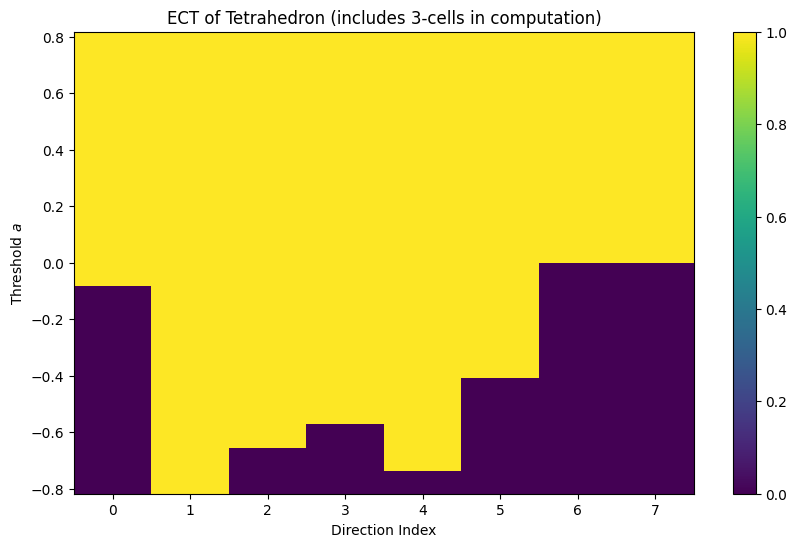
3.1.3. ECT Computation with Higher-Dimensional Cells

The ECT computation now properly includes all cell dimensions in the Euler characteristic calculation:

χ = Σ(-1)^k × |k-cells below threshold|

Let’s see how this works:

# Compute ECT for the tetrahedron
ect = ECT(num_dirs=8, num_thresh=20)
result = ect.calculate(K_tetra)

print(f"ECT result shape: {result.shape}")
print(f"Directions: {len(result.directions)} directions in {K_tetra.dim}D")
print(f"Thresholds: {len(result.thresholds)} threshold values")

# Plot the ECT matrix
fig, ax = plt.subplots(figsize=(10, 6))
result.plot()
plt.title('ECT of Tetrahedron (includes 3-cells in computation)')
plt.show()

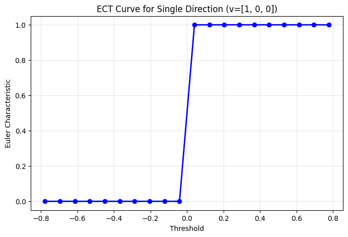
single_direction = ECT(num_thresh=20, directions=Directions.from_vectors([[1, 0, 0]])).calculate(K_tetra)
fig, ax = plt.subplots(figsize=(8, 5))
ax.plot(single_direction.thresholds, single_direction[0], 'b-', marker='o', linewidth=2)
ax.set_xlabel('Threshold')
ax.set_ylabel('Euler Characteristic')
ax.set_title('ECT Curve for Single Direction (v=[1, 0, 0])')
ax.grid(True, alpha=0.3)
plt.show()

ECT result shape: (8, 20)
Directions: 8 directions in 3D
Thresholds: 20 threshold values

3.1.4. Validation System

Sometimes we need our EmbeddedComplex to satisfy certain constraints such as no-self intersections. You can enforce these constraints using

K_tetra.enable_embedding_validation()
#add intersecting edge
K_tetra.add_node("E", [0.5,0,0])
try:
    K_tetra.add_cell(["A", "B"], dim=1, check=True)
except Exception as e:
    print(e)
    print("adding intersecting edge failed")

K_tetra.disable_embedding_validation()
K_tetra.add_cell(["A", "B"], dim=1)

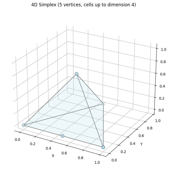
print("4D Simplex Cell Counts:")
for dim in sorted(K_tetra.cells.keys()):
    print(f"  {dim}-cells: {len(K_tetra.cells[dim])}")

# Plot (showing 3D projection)
fig = plt.figure(figsize=(10, 8))
ax = fig.add_subplot(111, projection="3d")
K_tetra.plot(ax=ax, face_alpha=0.1, node_size=80)
ax.set_title("4D Simplex (5 vertices, cells up to dimension 4)")
plt.show()

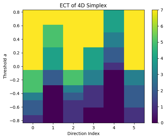
# Compute ECT
ect_4d = ECT(num_dirs=6, num_thresh=15)
result_4d = ect_4d.calculate(K_tetra)

result_4d.plot()
plt.title("ECT of 4D Simplex")
plt.show()

Edge Interior Validation: Vertex 4 lies on edge interior
adding intersecting edge failed
4D Simplex Cell Counts:
  1-cells: 1
  2-cells: 4
  3-cells: 1